Lab 10 Extra: Blocks

Sometimes it is revealing to group the nodes of a network according to the types of connections they have. Group-membership data suggests a natural grouping: two people are of the same type if they belong to exactly the same groups. Han refers to this grouping as “‘structually equivalent’ blocks in the person-to-person network” (154) and produces two pictures of this blocking for the data about Boston revolutionaries: figure 1 and figure 4. The idea is to pull together all the nodes in a block and show the number of ties this block has to each of the others.

Notice that a block is not the same as a clique or neighborhood or any other type of closely-connected set of nodes. In this case, it is true, nodes in any block are connected by their shared memberships, but many such nodes also have connections out of the block to other blocks (see the figure below). In some other kinds of networks, by contrast, a blocking may be possible in which the nodes in a block are not connected to each other at all.¹

Let’s begin with the same setup as Lab 10.

library(dataculture)
library(igraph)
library(ggraph)
library(tidygraph)

# Keep only the membership groups
whig_han <- whigs[ , -c(5, 7)]
# keep rows whose sum is strictly positive
whig_han <- whig_han[rowSums(whig_han) > 0, ]
# Compute the person-to-person graph
P <- whig_han %*% t(whig_han)
wp <- graph_from_adjacency_matrix(P, weighted="strength", mode="undirected")

Though identifying blocks in networks can be a complex endeavor in general, in this case, the membership blocks are right there to consider. It’s only a matter of data wrangling to reproduce Han’s blocking. Unfortunately the wrangling is fiddly. Here is a moderately cutesy approach that takes advantage of the fact that the affiliation matrix entries are only 0 or 1. We can encode each row as a single binary number, so the possible affiliation combinations have values of (decimal) 0 to 31. This encoding can be calculated by multiplying the affiliation matrix on the right by a column vector whose elements are the powers of two.² With the result, we can use the igraph function contract to glomp together all the vertices with the same block number. The glomping leaves many edges between each of the blocks, so we use igraph’s simplify to turn these into single weighted edges.

# calculate block numbers: binary encoding
whig_blocks <- whig_han %*% 2^(0:4) 
# now contract the graph
whig_blocks_net <- wp |>
    contract(whig_blocks, vertex.attr.comb="ignore") |>
    set_edge_attr("weight", value=1) |>
    simplify(edge.attr.comb="sum")

This network can be visualized as follows:

ggraph(whig_blocks_net, layout="mds") +
    geom_node_point(aes(filter=centrality_degree() > 0)) +
    geom_edge_fan()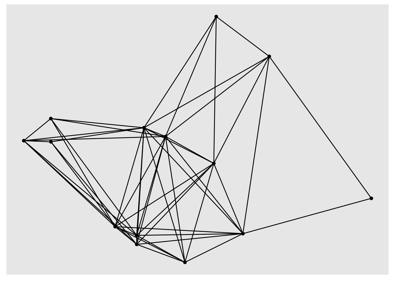

The layout="mds" is “multidimensional scaling,” yet another approach to putting networks on the plane that tries to put closely-connected vertices near each other. This is the method Han uses for his fig. 4. The filter clause is a special “aesthetic” which removes nodes with no neighbors (the blocks corresponding to the many individuals in only one group).

But this network of blocks is I think harder to read by eye than Han’s fig. 1, which shows the same blocking in grid form. In class I showed a remake of this figure. Mine is not as elegant as Han’s—it lacks the thin lines indicating all the connections among the blocks—but it does show you the kind of tedious data-wrangling code you need to be able to look visually at a matrix like this. The plot doesn’t use any igraph or ggraph stuff, just a bunch of data-frame manipulation and a heap of ggplot fiddling:

as_tibble(whig_han, rownames="name") |>
    # sort by group memberships, then by name
    arrange(across(c(2:6, 1))) |>
    # make `name` a factor with this ordering
    mutate(name=factor(name, levels=name, ordered=T)) |>
    # create one row for each person-group pair
    pivot_longer(-1, names_to="group", values_to="belongs") |>
    # flag people with >= 3 memberships
    group_by(name) |>
    # tally memberships 
    mutate(memberships=sum(belongs)) |>
    ungroup() |>
    # recode group names (chron. order)
    mutate(group=fct_recode(group,
        "St. Andrews Lodge\n1762"="St Andrews Lodge",
        "Loyal Nine\n1766"="Loyal Nine",
        "North End Caucus\n1771"="North Caucus",
        "Long Room Club\n1773"="Long Room Club",
        "Boston Committee\n1774"="Boston Committee")) |>
    ggplot(aes(x=name, y=group)) + 
        geom_tile(aes(alpha=as.logical(belongs), fill=memberships)) +
        scale_x_discrete(labels=NULL) +
        scale_alpha_manual(values=0:1, guide="none") +
        # seems to produce three bins, 1-2, 3, 4, by default
        scale_fill_binned(type = "viridis", guide="none") +
        theme_void() +
        theme(axis.text.y=element_text(
                 hjust=1,
                 margin=margin(0, 4, 0, 0)),
              legend.position="bottom",
              plot.margin = margin(10, 10, 0, 10))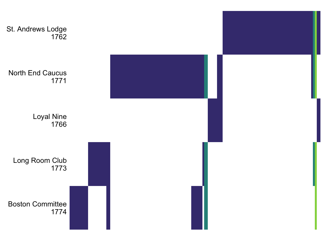

Blocks corresponding to people with more group memberships are highlighted by color. There are only 4 people with at least three memberships. We can pick them out out of the affiliation matrix:

whig_han[rowSums(whig_han) >= 3, ] |>
    knitr::kable()

	St Andrews Lodge	Loyal Nine	North Caucus	Long Room Club	Boston Committee
Samuel Adams	0	0	1	1	1
Benjamin Church	0	0	1	1	1
Paul Revere	1	0	1	1	0
Joseph Warren	1	0	1	1	1

Han’s point is that though Samuel Adams and Benjamin Church spanned three groups, they didn’t act as bridges to the St. Andrew’s Lodge group the way Revere and Warren did. St. Andrew’s Lodge is important to Han’s argument because, as he shows, it was particularly associated with the group of artisans and farmers—people of lower (or “middling”) social status, who also formed the rank-and-file of the Minutemen (155–56).

Benjamin Church was a name I didn’t know; he turns out to have been a British spy (see Fischer, Paul Revere’s Ride, 38, 51–52). That gives you another type of person who is likely to be found in a bridging or “brokerage” role in revolutionary networks.