Lab 8 Bonus: Logistic regression modeling machinery

For the statisticurious, here are a few further notes on Underwood’s genre-modeling techniques. The following material is completely optional and not at all required or significant for Paper 2. I will assume some familiarity with some regression modeling/machine learning terms.

Underwood’s genre models in Distant Horizons are regularized logistic regression models. These are simple to generate with R, though the underlying algorithms are not all simple. Using these tools for a polished analysis entails quite a few subtleties. Nonetheless, I thought I would give a little flavor of these things.

library(dataculture)
library(Matrix)
# more utility functions
library(broom)

Note to visitors in 2023 and after: since I updated my dataculture package, to run the code below you will also need to explicitly load the tidyverse:

library(tidyverse)

Logistic regression without regularization is built into R, as an application of the glm function. For example, imagine we were interested in using just a small number of features to guess genre. Let’s repeat the lab setup.

n_sf <- genre_meta |>
    filter(str_detect(tags, "scifi")) |>
    nrow()
meta_sf <- genre_meta |>
    select(docid, author, title, firstpub, tags) |>
    mutate(sf=str_detect(tags, "scifi"),
           random=str_detect(tags, "random") & !sf)
sf_set <- meta_sf |>
    filter(sf | random) |>
    group_by(sf) |>
    # randomly choose n_sf random volumes
    # (and n_sf SF volumes, but that's all of them)
    slice_sample(n=n_sf) |>
    ungroup()

We estimated one-regressor models by eye in the lab. Here’s how to do it by machine:

sf_space <- sf_set |>
    mutate(space=genre_features[docid, "space"])

m1 <- glm(data=sf_space, formula=sf ~ space, family="binomial")

This computes the maximum-likelihood estimate of the logistic regression model. R uses special classes of data to represent statistical models, together with specialized functions for manipulating them. I’ll be throwing those around without explanation here. The fitted model is:

tidy(m1) |> select(term, estimate, std.error) |>
    knitr::kable(digits=2)

term	estimate	std.error
(Intercept)	-1.3	0.17
space	11706.2	1650.54

The 0.5-probability threshold for guessing “SF” occurs when the linear predictor is exactly zero, which in this case occurs at

-coef(m1)["(Intercept)"] / coef(m1)["space"]

##  (Intercept) 
## 0.0001108211

Here is what a logistic regression model with just a few more features looks like:

sf_feats <- sf_set |>
    mutate(space=genre_features[docid, "space"],
           time=genre_features[docid, "time"],
           alien=genre_features[docid, "alien"])

m2 <- glm(data=sf_feats, formula=sf ~ space + time + alien, family="binomial")

tidy(m2) |> select(term, estimate, std.error) |>
    knitr::kable(digits=2)

term	estimate	std.error
(Intercept)	-1.71	0.49
space	9715.13	1635.70
time	143.24	262.89
alien	20720.17	5337.32

Its in-sample classification performance can be computed by finding the fitted probabilities:

augment(m2, type.predict="response") |>
    summarize(correct=mean((.fitted > 0.5) == sf))

## # A tibble: 1 × 1
##   correct
##     <dbl>
## 1   0.773

Classifiers should, however, always be checked on out-of-sample performance. Let’s not belabor this on the toy model but move on to regularization, which will allow us to use as many features as Underwood does.

As we noted in the lab, Underwood works with thousands of features for each document he models. When we have more features than cases, logistic regression, like linear regression, degenerates: we can no longer estimate a “best fit” since there are infinitely many models with ostensibly perfect fits. We need some way to avoid creating a classifier that “memorizes” all of its training data and misleads us into thinking it is better than it really is. An overfitted model looks good on training data but does poorly on new data. Regularization reduces overfitting by imposing limits on how much we allow any one variable to matter in the model: as statisticians put it, it trades bias for variance.

Regularized logistic regression in R is carried out with the glmnet package. This can installed with

install.packages("glmnet")

library(glmnet)

A regularized fit similar to those Underwood discusses can be computed with a single function call:

m3 <- glmnet(x=genre_features[sf_set$docid, ], y=sf_set$sf, family="binomial",
             alpha=0, standardize=T)

alpha=0 means this does a “ridge regression” or “L2 regularization.” The resulting m3 is actually a list of models fitted at varying values of the regularization parameter \(\lambda\); the bigger \(\lambda\) is, the stronger the regularization. By default glmnet tries 100 \(\lambda\) values. Here is a chart of their in-sample accuracies:

m3_insample <- predict(m3, newx=genre_features[sf_set$docid, ], type="class")
tibble(lambda=m3$lambda,
    accuracy=apply(m3_insample, 2,
                   function (preds) mean(preds == sf_set$sf)
    )) |>
    ggplot(aes(lambda, accuracy)) + geom_line()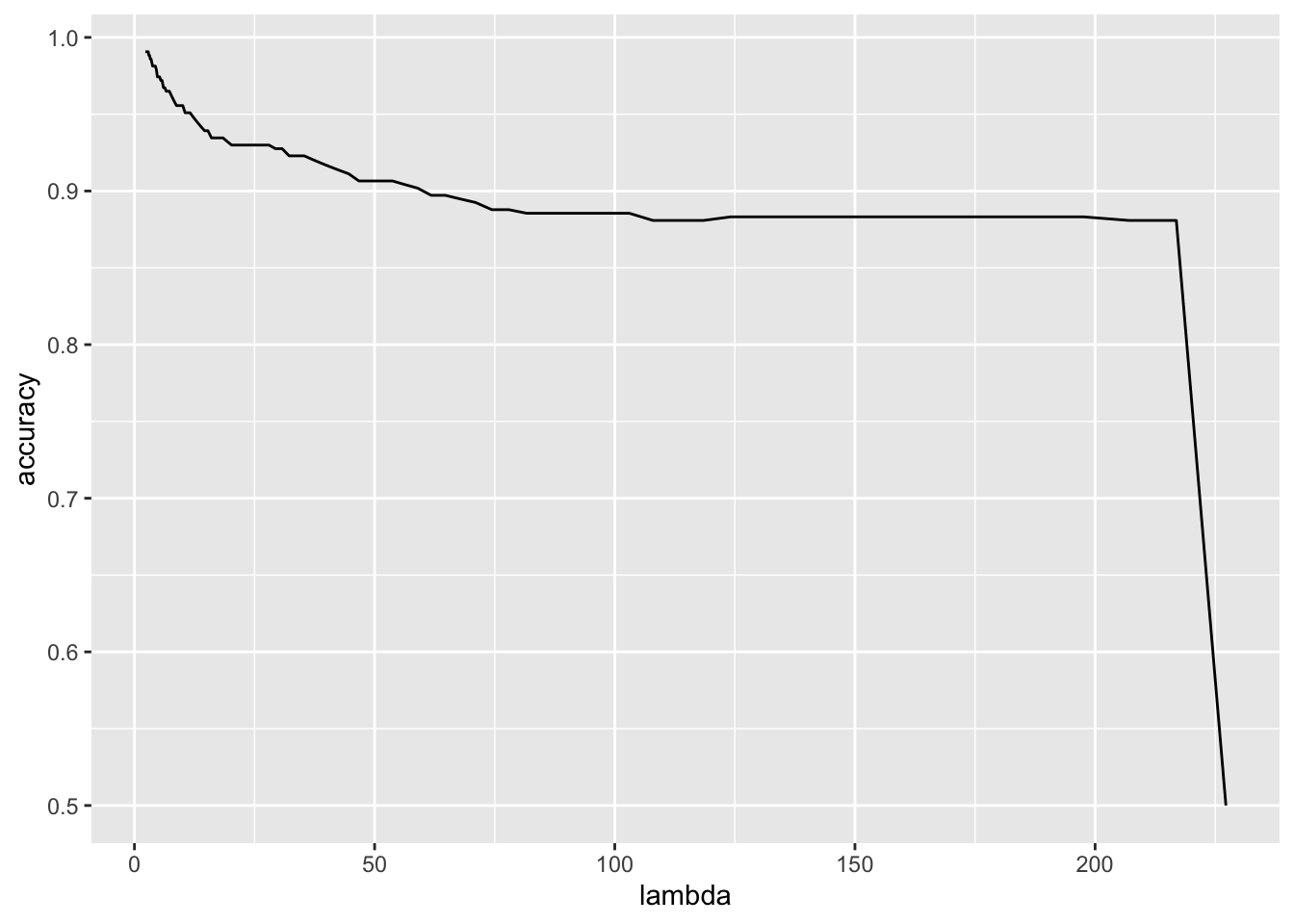

At the minimal (non-zero) \(\lambda\) value, the model is pretty much perfect on its training data, but this is pure overfitting. In-sample accuracy is a misleading measure, even with regularization applied. We should (as Underwood does) try to get a model that performs better on unseen data by using cross-validation. glmnet wraps up cross-validation for us in another convenient one-liner:

m4 <- cv.glmnet(x=genre_features[sf_set$docid, ], y=sf_set$sf, family="binomial",
             alpha=0, standardize=T, nfolds=10, type.measure="class",
    trace.it=1 # show progress bar
)

On my laptop—a fairly powerful Macbook Pro—there is a noticeable wait (15 sec) to finish this computation. m4 again returns a list of models estimated at varying \(\lambda\) values, but now at each of those values the estimate is nfolds-fold cross-validated. Cross-validation allows us to consider a less biased estimate of the out-of-sample classification performance of the modeling process:¹

1 - min(m4$cvm)

## [1] 0.9088785

and this is estimated to have a standard deviation of

m4$cvsd[which.min(m4$cvm)]

## [1] 0.01360653

This is still pretty good, and unlike the near-perfect in-sample accuracy of m2, likely closer to how our classifier would really perform on an entirely unseen corpus of texts with comparable genre labeling. Some coefficients of the features can be extracted with

coef(m4, s="lambda.min")[ , 1] |> sort(decreasing=T) |> head(10)

##     blocked      ignore     horrors      varied     wasting       scrap 
##    410.8120    402.4308    394.1365    391.9441    386.2260    384.5504 
##       dazed   nightmare     shudder combination 
##    370.3737    365.7563    359.0826    356.1798

coef(m4, s="lambda.min")[ , 1] |> sort() |> head(10)

##    shrewd    boldly   propped       sly    bolted  marrying    gossip    shabby 
## -495.9137 -485.5515 -468.1274 -465.9627 -458.4750 -450.5228 -448.0896 -447.3250 
##  defiance    smoked 
## -435.8537 -433.4834

Because we used ridge regression with alpha=0, all 4889 features are used in the model.

Underwood’s technique is a little more refined that what I have just demonstrated. It is well known that bags of words produced from different texts by the same author tend to be quite highly correlated (this fact can even be used to detect authorship in anonymous texts). We may still have a significant bias in our estimate of how well our model performs, if we are getting an “unfair” advantage from recognizing individual authors who recur in the set. (Then again, it’s not completely clear to me we always want the “fair” version, since genres are sometimes dominated by certain authors, at least for a time, and our model ought to capture that.) Underwood goes to some lengths to avoid testing a model on data produced by the same author it was trained on. This takes a little finesse if we don’t want to waste any data, and I won’t go through that here.² A simpler approach is to ensure we only have one title by any given author in our set. That can be done with a few quick manipulations:

sf_set2 <- meta_sf |>
    group_by(author) |>
    slice_sample(n=1) |>
    filter(sf | random)
n_sf2 <- sum(sf_set2$sf)
sf_set2 <- sf_set2 |>
    group_by(sf) |>
    slice_sample(n=n_sf2) |>
    ungroup()

We have only half as much data this way (135 SF and non-SF texts each), so the comparison with the earlier models won’t be perfect. But let’s try the model and see how we do:

m5 <- cv.glmnet(x=genre_features[sf_set2$docid, ], y=sf_set2$sf, family="binomial",
             alpha=0, standardize=T, nfolds=10, type.measure="class")

I was rather surprised to find that this does quite as well:

1 - min(m5$cvm)

## [1] 0.9259259

with a standard error of

m5$cvsd[which.min(m5$cvm)]

## [1] 0.01352401

An Underwood-esque plot would look like

sf_set2 |> mutate(
    pred=predict(m5, newx=genre_features[sf_set2$docid, ],
                 type="response", s="lambda.min")) |>
    ggplot(aes(firstpub, pred, color=sf)) + geom_point(alpha=0.5)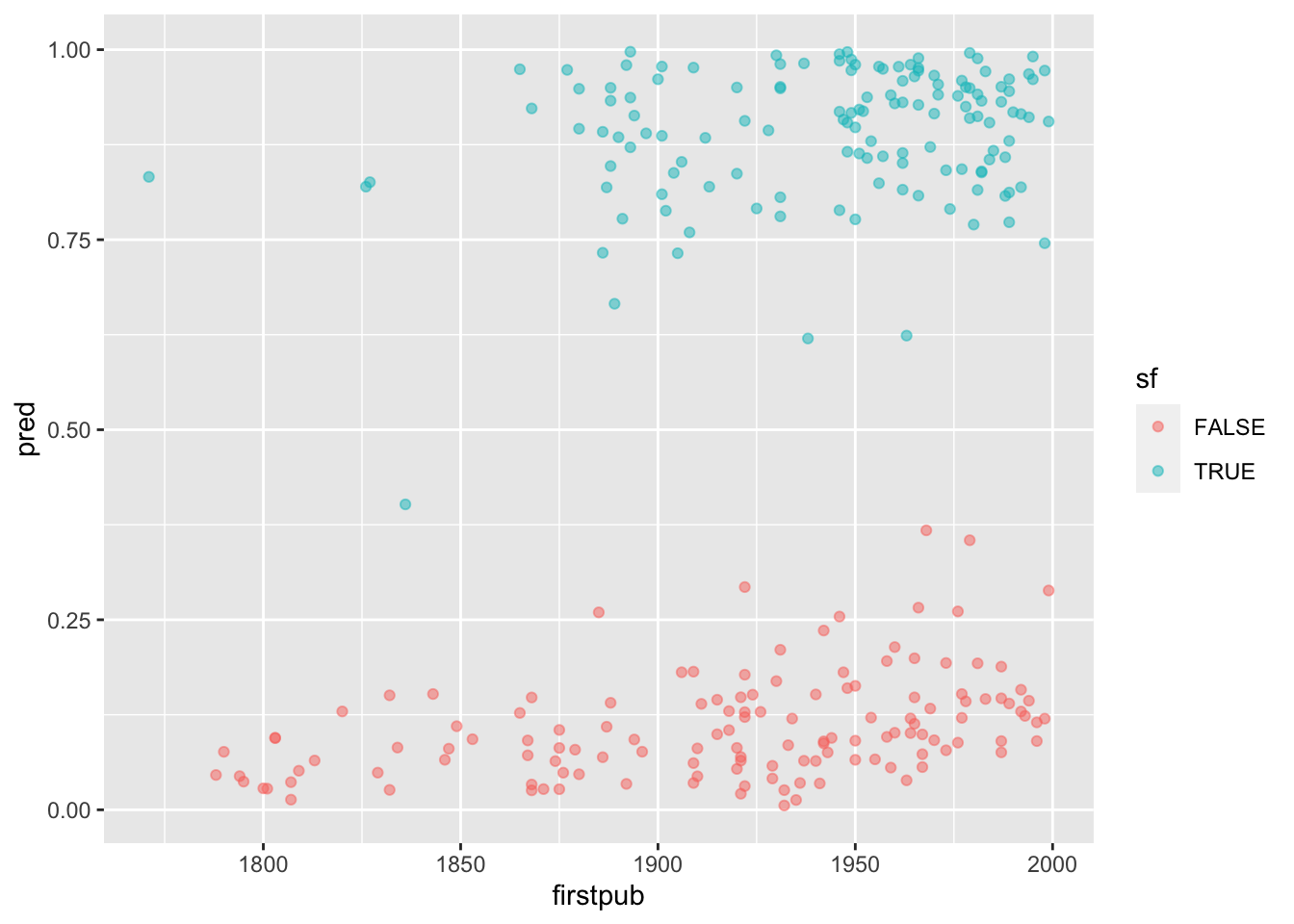

In-sample, this classifier is nearly perfect—but notice that the cross-validated estimate of out-of-sample performnace is in the same 91% vicinity Underwood reports. And because the “best” \(\lambda\) is very small, we should continue to suspect overfitting.

Let’s try a variation in the approach. Underwood relies on the most classic form of regularized regression, the “ridge.” glmnet makes it easy to try another possibility, the “lasso” or “L1 regularization,” which is a strategy that is said to “select features” by forcing many coefficients to exactly 0. glmnet also lets you use a compromise between the two strategies, the so-called “elastic net.” The choice is controlled by the alpha parameter to glmnet and cv.glmnet. Here is the lasso, alpha=1:

m6 <- cv.glmnet(x=genre_features[sf_set2$docid, ], y=sf_set2$sf, family="binomial",
             alpha=1,
             standardize=T, nfolds=10, type.measure="class")

This is noticeably faster than the ridge, which can be an advantage on bigger datasets. Its classification performance

1 - min(m6$cvm)

## [1] 0.8888889

(SE: 0.0206583) is slightly worse, but, as is characteristic of the lasso, it sends most coefficients to zero. The model has only

m6$nzero[which.min(m6$cvm)]

## s42 
##  81

non-zero coefficients at the optimal \(\lambda\) value. If we tolerate one standard deviation of inaccuracy more, we can eliminate almost all features. The number of non-zero features in that model is

m6$nzero[m6$lambda == m6$lambda.1se]

## s20 
##  30

This set is interesting to look at, though it is not a definitive finding: there is some uncertainty in which features come up non-zero when you use the lasso, and some randomness introduced through cross-validiation. Indeed, each time I re-run the code in this post, I get a different list (and different numbers too).

m6_coefs_1se <- coef(m6, s="lambda.1se")[ , 1]
tibble(feature=names(m6_coefs_1se), coefficient=m6_coefs_1se) |>
    filter(coefficient != 0) |>
    arrange(desc(coefficient)) |>
    knitr::kable(digits=2)

feature	coefficient
thousands	2367.22
larger	2211.79
automatically	2102.29
ability	1867.33
relax	1649.53
machinery	1373.18
nearest	1313.00
contact	784.71
able	584.15
surface	570.19
function	525.97
human	491.63
problem	486.14
metal	356.62
structure	247.09
its	221.26
complex	125.20
waved	57.87
power	34.66
earth	5.93
(Intercept)	-0.42
young	-34.61
letter	-42.39
who	-122.04
affection	-181.46
#dayoftheweek	-249.17
temper	-351.86
hat	-496.43
favourite	-598.83
tea	-1358.78
married	-2589.05

Finally, this machinery makes it simpler to try Underwood’s investigative strategy of modeling one chronological slice of the data and testing the model on a later slice. Here is an example that splits things at 1935. I’ll go back to allowing repeat authors.

sf_pre35 <- meta_sf |>
    filter(firstpub <= 1935) |>
    ungroup() |>
    filter(sf | random)
n_pre35_sf <- sum(sf_pre35$sf)
sf_pre35 <- sf_pre35 |>
    group_by(sf) |> 
    slice_sample(n=n_pre35_sf) |>
    ungroup()

m7 <- cv.glmnet(x=genre_features[sf_pre35$docid, ], y=sf_pre35$sf, family="binomial",
             alpha=1, standardize=T, nfolds=10, type.measure="class")

This is a fairly high-performing model

1 - min(m7$cvm)

## [1] 0.95

(SE: 0.0181621), and does remarkably well retrodicting the subsequent “future” of the genre:

sf_post35 <- meta_sf |>
    filter(firstpub <= 1935) |>
    ungroup() |>
    filter(sf | random)
n_post35_sf <- sum(sf_post35$sf)
sf_post35 <- sf_post35 |>
    group_by(sf) |> 
    slice_sample(n=n_post35_sf) |>
    ungroup()

sf_post35 |>
    mutate(pred=predict(m7, newx=genre_features[sf_post35$docid, ], s="lambda.min",
                        type="response")) |> 
    summarize(accuracy=mean((pred > 0.5) == sf))

## # A tibble: 1 × 1
##   accuracy
##      <dbl>
## 1     0.95

Underwood goes on to vary the chronological cutoff point, and you should be able to imagine other experiments using different slices of the metadata. But before you go into business as a consulting genre detective, go think about the conceptual issues Paper 2 asks you to.