Names and mining strategies

The final, “bonus” part of Lab 6 was an exploration of names that were more prominent in NJ than nationally. In the visualization I used the ratio of names’ frequency in the state to their national frequency to pick out these names. But one issue with this ratio measure is that it does not distinguish more common from very uncommon names. A name that occurs 2 in 10000 times in NJ and 1 in 10000 times nationally scores the same as one which occurs 200 in 10000 times in NJ and 100 in 10000 times nationally. Yet, intuitively, the latter seems far more significant. One way to quantify this intuition is to develop a very simple statistical model and use it to assess which names are exceptional. Here is one such approach, based on the likelihood-ratio statistic, inspired by a technique from text mining, described in Ted Dunning’s “Accurate Methods for the Statistics of Surprise and Coincidence,” for identifying “distinctive” phrases in documents. The rest of this post won’t make total sense unless you know what a binomial distribution and a likelihood ratio are, so I guess it’s for the statisticurious.¹ If you are statisticurious, I think it’s often a good idea to reflect on what the statistical assumptions behind an exploration are—one is never really “just looking” but always using some kind of implicit model.

The model here is that, for any given year, any given US state, any given name, and any given sex, there is a fixed probability that each new baby will receive the name. And all the probabilities of other names are completely independent.² Let us say, in 2019, for every baby boy born in NJ, there was some fixed probability \(p\) its parents would give him the name Joseph. The resulting counts of baby names are modeled as the results of binomial trials, so the probability of getting a given number \(k\) of boys named Joseph if a total of \(n\) boys are born is the binomial probability

\[ {n \choose k} p^k (1 - p)^k \]

We can estimate this probability \(p\) by the proportion of baby boys named Joseph in NJ in that year:

library(dataculture)

Note to visitors in 2023 and after: since I updated my dataculture package, to run the code below you will also need to explicitly load the tidyverse:

library(tidyverse)

## ── Attaching core tidyverse packages ──────────────────────── tidyverse 2.0.0 ──
## ✔ dplyr     1.1.2     ✔ readr     2.1.4
## ✔ forcats   1.0.0     ✔ stringr   1.5.0
## ✔ ggplot2   3.4.2     ✔ tibble    3.2.1
## ✔ lubridate 1.9.2     ✔ tidyr     1.3.0
## ✔ purrr     1.0.1     
## ── Conflicts ────────────────────────────────────────── tidyverse_conflicts() ──
## ✖ dplyr::filter() masks stats::filter()
## ✖ dplyr::lag()    masks stats::lag()
## ℹ Use the conflicted package (<http://conflicted.r-lib.org/>) to force all conflicts to become errors

nj19 <- recent_ssa_state_names |> filter(state == "NJ", year == 2019) |>
    select(sex, name, k_nj=n, p_nj=prop)
us19 <- recent_ssa_names |> filter(year == 2019) |>
    select(sex, name, k_us=n, p_us=prop)

nj19 |> filter(sex == "M", name == "Joseph") |> 
    pull(p_nj)

## [1] 0.008506985

Now we construct a test of the null hypothesis that being born in NJ and being named Joseph are independent events, that is to say that the NJ-specific probability is the same as the probability everywhere else in the US, against the alternative these two probabilities differ. This can be formulated as a likelihood ratio test. It is not too hard to derive the likelihood ratio (see Dunning), which is

\[ \lambda = \frac{p^{k_1} (1 - p)^{k_1} p^{k_2} (1-p)^{k_2}} {p_1^{k_1} (1 - p_1)^{k_1} p_2^{k_2} (1-p_2)^{k_2}} \]

where \(p_1 = k_1 / n_1\), \(p_2 = k_2 / n_2\), and \(p = (k_1 + k_2) / (n_1 + n_2)\), with \(k_1\) the number of NJ Josephs, \(n_1\) the number of NJ boys, \(k_2\) the number of non-NJ Josephs, and \(n_2\) the number of non-NJ boys. The test statistic is \(-2\log\lambda\), and for our purposes all that matters is that this statistic will be large for large violations of the null hypothesis.³

With that preamble, we can define our magic “distinctiveness” score with the following R functions:

ll <- function (p, k, n) k * log(p) + (n - k) * log(1 - p)

G <- function (p1, k1, n1, p2, k2, n2, p) {

    2 * (ll(p1, k1, n1) + ll(p2, k2, n2) -
    ll(p, k1, n1) - ll(p, k2, n2))
}

# wastefully recover the totals by dividing back out, shrug
nj19_scored <- nj19 |> inner_join(us19, by=c("name", "sex")) |>
    mutate(n_nj = k_nj / p_nj, n_us = k_us / p_us) |>
    mutate(n_non = n_us - n_nj, k_non = k_us - k_nj,
           p_non = k_non / n_non) |>
    mutate(g = G(p1=p_nj, k1=k_nj, n1=n_nj,
                 p2=p_non, k2=k_non, n2=n_non, p=p_us))

The top results here correspond with our previous analysis. I’ll show proportions per 1000:

nj19_scored |> slice_max(g, n=40) |>
    select(name, k_nj, p_nj, k_us, p_us, g) |>
    mutate(p_nj = p_nj * 1000, p_us=p_us * 1000) |>
    knitr::kable(digits=1)

name	k_nj	p_nj	k_us	p_us	g
Rivka	134	2.8	381	0.2	493.3
Chana	119	2.5	353	0.2	426.5
Moshe	141	2.8	553	0.3	416.1
Rochel	75	1.6	131	0.1	369.4
Yehuda	97	1.9	268	0.1	361.3
Shmuel	84	1.6	202	0.1	340.7
Yisroel	91	1.8	250	0.1	340.1
Chaim	104	2.0	359	0.2	335.2
Shlomo	81	1.6	197	0.1	326.3
Tzvi	75	1.5	170	0.1	315.2
Yaakov	73	1.4	160	0.1	313.0
Yosef	101	2.0	390	0.2	301.3
Chaya	99	2.0	440	0.2	268.8
Malka	67	1.4	181	0.1	254.6
Dovid	58	1.1	127	0.1	248.8
Avrohom	51	1.0	91	0.0	246.8
Mordechai	79	1.5	294	0.2	241.8
Shoshana	58	1.2	138	0.1	238.1
Nechama	52	1.1	103	0.1	237.9
Miriam	139	2.9	1161	0.6	214.5
Meir	62	1.2	197	0.1	211.1
Yitzchok	56	1.1	186	0.1	185.2
Eliyahu	47	0.9	119	0.1	184.7
Esther	158	3.3	1727	0.9	175.8
Avraham	51	1.0	167	0.1	170.2
Aryeh	46	0.9	134	0.1	165.7
Batsheva	36	0.7	73	0.0	162.5
Yehudis	34	0.7	75	0.0	146.0
Sara	144	3.0	1740	1.0	138.8
Dov	41	0.8	134	0.1	137.0
Ahron	29	0.6	57	0.0	132.6
Baila	40	0.8	134	0.1	132.4
Joseph	436	8.5	9125	4.8	127.3
Nicholas	262	5.1	4626	2.4	121.4
Yehoshua	33	0.6	95	0.0	119.7
Bracha	31	0.6	83	0.0	118.4
Devorah	37	0.8	131	0.1	118.0
Ryan	317	6.2	6108	3.2	117.7
Waylon	11	0.2	3433	1.8	116.9
Nosson	23	0.4	39	0.0	114.7

But we can see that the statistic does indeed focus attention on fairly frequent names, allowing us to catch the moderately exceptional frequency of Joseph, Nicholas, and Ryan in the state as well. The visualization, which reveals some more interesting possibilities for investigation among unusually uncommon names as well, might look like this:

nj19_scored |>
    ggplot(aes(p_nj, g, label=name, color=sex)) +
        geom_text() +
        scale_x_log10()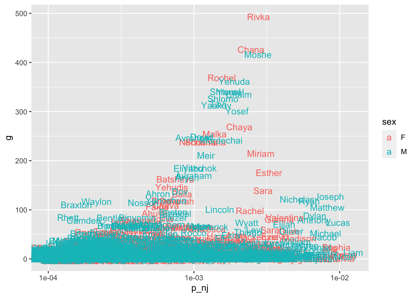

The log-likelihood ratio score here is related to two very-widely used “relevance” scoring techniques for text-database search results, mutual information and TF-idf weighting.

We could repeat the calculation for every state, producing a list of the most “distinctive” girl and boy names in 2019:

recent_ssa_state_names |> filter(year == 2019) |>
    select(sex, name, state, k_state=n, p_state=prop) |>
    inner_join(us19, by=c("name", "sex")) |>
    mutate(n_state = k_state / p_state, n_us = k_us / p_us) |>
    mutate(n_non = n_us - n_state, k_non = k_us - k_state,
           p_non = k_non / n_non) |>
    mutate(g = G(p1=p_state, k1=k_state, n1=n_state,
                 p2=p_non, k2=k_non, n2=n_non, p=p_us)) |>
    group_by(state, sex) |>
    slice_max(n=1, g) |>
    select(state, sex, name, p_state) |>
    mutate(p_state = p_state * 1000) |>
    knitr::kable(digits=1)

state	sex	name	p_state
AK	F	Aurora	7.2
AK	M	Hatcher	1.4
AL	F	Mary	5.3
AL	M	John	9.5
AR	F	Blakely	2.9
AR	M	Kingston	4.2
AZ	F	Ximena	3.1
AZ	M	Jesus	4.4
CA	F	Camila	9.5
CA	M	Mateo	9.7
CO	F	Aspen	2.5
CO	M	Nolan	5.2
CT	F	Gianna	4.9
CT	M	Luca	5.6
DC	F	Maya	8.7
DC	M	William	18.6
DE	F	Milan	1.6
DE	M	Colton	7.2
FL	F	Valentina	4.3
FL	M	Thiago	2.8
GA	F	Skylar	4.3
GA	M	Amir	3.3
HI	F	Mahina	2.5
HI	M	Kaimana	2.1
IA	F	Cora	4.3
IA	M	Kinnick	0.7
ID	F	Oakley	3.1
ID	M	Ridge	2.0
IL	F	Maeve	1.8
IL	M	Mateo	6.9
IN	F	Camila	1.8
IN	M	Lincoln	6.8
KS	F	Hadley	3.8
KS	M	Brooks	4.3
KY	F	Camila	0.8
KY	M	Waylon	6.2
LA	F	Camille	2.9
LA	M	Mateo	1.2
MA	F	Maeve	3.6
MA	M	Benjamin	13.5
MD	F	Genesis	4.7
MD	M	Emiliano	0.3
ME	F	Eleanor	8.4
ME	M	Owen	12.3
MI	F	Camila	1.1
MI	M	Ali	2.4
MN	F	Maida	0.7
MN	M	Abdirahman	1.4
MO	F	Camila	1.2
MO	M	Mateo	1.5
MS	F	Camila	0.4
MS	M	Mateo	0.8
MT	F	Aspen	3.5
MT	M	Colter	2.5
NC	F	Caroline	4.1
NC	M	Bryson	3.7
ND	F	Girl	1.2
ND	M	Boy	1.5
NE	F	Sutton	2.2
NE	M	Barrett	4.0
NH	F	Charlotte	16.0
NH	M	Owen	12.2
NJ	F	Rivka	2.8
NJ	M	Moshe	2.8
NM	F	Zia	1.8
NM	M	Ezekiel	7.0
NV	F	Caroline	0.5
NV	M	Romeo	1.7
NY	F	Chaya	2.4
NY	M	Moshe	3.0
OH	F	Camila	1.1
OH	M	Mateo	1.2
OK	F	Gentry	0.8
OK	M	Baker	2.7
OR	F	Unknown	1.2
OR	M	Unknown	1.4
PA	F	Camila	1.5
PA	M	Santiago	0.5
RI	F	Grace	7.8
RI	M	Julian	10.8
SC	F	Sofia	1.1
SC	M	Kingston	4.8
SD	F	Shay	1.6
SD	M	Briggs	3.6
TN	F	Everleigh	3.4
TN	M	Waylon	4.7
TX	F	Camila	9.0
TX	M	Jose	5.8
UT	F	Navy	2.8
UT	M	Boston	2.6
VA	F	Virginia	1.2
VA	M	William	10.4
VT	F	Harper	13.0
VT	M	Emmett	7.6
WA	F	Juniper	2.1
WA	M	Emmett	3.5
WI	F	Nora	5.9
WI	M	Owen	8.6
WV	F	Paisley	7.9
WV	M	Braxton	7.8
WY	F	Willow	6.9
WY	M	Bridger	2.7

And I could now produce one of those annoying “characterize your state by some thing that’s especially popular in it” graphics, but I won’t. Plus the Oregonians would be mad about “Unknown” and the North Dakotans would probably say passive-aggressive things about “Girl” and “Boy.”