Nobel Literature Prizes - Data and Culture

My other first-day-of-class example was based on information about the Nobel Prize in Literature. The Swedish Academy (which awards the prize) has loads of information about the literature prizewinners on its website. In fact they even have an API that allows programmatic access to a database about all the Nobel laureates, which returns results in JSON. However, this API is a lot harder to use than the handy table on Wikipedia. I thought I should record how I scraped that table and made my plot of Nobel literature languages.

When you get data from the web, I highly recommend storing a local copy rather than assuming that a given website will always be acccessible (and that what’s on it won’t change). Wikipedia can be changed by anyone, though it is quite reliable for things like this, which are easily cited to an authoritative source on the web. The really interesting aspect of the data-generating process is the social/cultural process that leads to the awarding of prizes to one writer or another. That’s what we want to study here.

But for now, let’s just look at getting the data. Here’s a simple way to download a webpage and store a local copy. First we have some libraries to invoke.

library(tidyverse)
library(rvest)

Then we get the relevant file and save it.

laureates_url <- "https://en.wikipedia.org/wiki/List_of_Nobel_laureates_in_Literature"
laureates_file <- "wiki-laureates.html"
# read_lines can read from a file on disk or from a URL
wiki_page <- read_lines(laureates_url)
# write_lines saves a file on disk
write_lines(wiki_page, laureates_file)

The HTML of the Wikipedia page is fairly easy to scrape. In this course we’ll skim over the details of how you do this, but just to show that it isn’t magic, here is the code, which uses functions from the rvest package:

laureates <- read_html(laureates_file) |>
    # select the first table element
    html_node("table") |>
    # convert to an R tibble
    html_table(fill=T) |>
    # remove the picture column
    select(-Picture) |>
    # neater column names
    rename(year=Year, genre=`Genre(s)`, language=`Language(s)`)

The resulting table reproduces the Wikipedia one in an R-friendly data structure:

head(laureates)

## # A tibble: 6 × 6
##    year Laureate                           Country       language Citation genre
##   <int> <chr>                              <chr>         <chr>    <chr>    <chr>
## 1  1901 Sully Prudhomme  (1839–1907)       France        French   "\"in s… poet…
## 2  1902 Theodor Mommsen  (1817–1903)       Germany       German   "\"the … hist…
## 3  1903 Bjørnstjerne Bjørnson  (1832–1910) Norway        Norwegi… "\"as a… poet…
## 4  1904 Frédéric Mistral  (1830–1914)      France        Provenç… "\"in r… poet…
## 5  1904 José Echegaray  (1832–1916)        Spain         Spanish  "\"in r… drama
## 6  1905 Henryk Sienkiewicz  (1846–1916)    Poland( Russ… Polish   "\"beca… novel

This too can be saved to disk for later exploration with

write_tsv(laureates, "literature-laureates.tsv")

and read back in with

laureates <- read_tsv("literature-laureates.tsv")

Because I create it here, you can download literature-laureates.tsv from this site.

All the columns here are interesting. In class on the first day, I showed some tallies of the laureates’ languages; here’s a slightly improved version. There’s some fiddly stuff in the code, some of the details of which I can’t promise to explain this semester. Making plots is always fiddly; in addition, I use a few tricks to manipulate the language column. But again, let’s at least show it’s not magic:

# plotting libraries
library(patchwork)

langs <- laureates |> select(year, language) |>
    # clean up language column: there are some years without a prize
    filter(language != "Not awarded") |>
    # and some laureates wrote in more than one language!
    # so we have to split and unnest
    mutate(language=str_split(language, " and ")) |>
    unnest(language) |>
    # convert language column to a factor ordered by frequency of levels
    # (factors are categorical variables)
    mutate(language=fct_infreq(language)) |>
    # make this order run from greatest to least
    mutate(language=fct_rev(language))

# create and store main plot with award year on x axis and language on y
lang_plot <- ggplot(langs, aes(year, language)) +
    geom_point(size=1) +
    scale_x_continuous(name="year of award",
        expand=expansion(mult=0.02), n.breaks = 12) +
    scale_y_discrete(name="", position="right")

# create and store "plot" of the totals for each language
lang_counts <- langs |>
    count(language) |>
    ggplot() +
        geom_text(x=0, aes(y=language, label=n), size=3) +
        scale_x_continuous(expand=expansion(add=1)) +
        theme_void()

# use patchwork "+" and plot_layout to put them together
print(lang_plot + lang_counts + plot_layout(widths=c(7, 1)))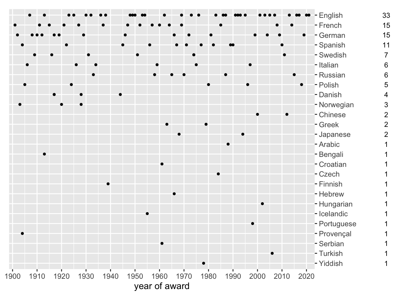

This table of laureates by itself is intriguing but provides only minimal evidence about the process that produces the Nobel laureates. An interesting further dataset is available from the Swedish academy, their Nomination archive, which gives information about people who were nominated for the Nobel prizes, whether they received it or not. The archive has information about the nominees up to 1971 (i.e. the past fifty years of nominees are still secret). Getting this information into a convenient form for analysis is less straightforward than the Wikipedia-scraping exercise above, but I can give some help if you’re interested.